Spilled array formulas (version -)

Summary

Dynamic array formulas that are spilling over the bordering cells are spilled array formulas. Since September 2018, this new feature is preferred to the legacy array formula.

In a nutshell, when using legacy array formulas, the user had to select the array or area over which the output was going to be mapped. After having entered the desired function in the top cell, the user had to hit Ctrl + Shift + Enter on his/her keyboard to get the results.

Spilled array formulas only require to enter the function with the correct input then the mapping is automatic.

#SPILL! errors

Errors can occur while using spilled array formulas which will transpire as such: #SPILL!. For more details, check out on the support.microsoft website.

Here is a list of the main reasons for an error message:

• Spill range is not blank
• Indeterminate size
• Extends beyond the worksheet’s edge
• Table formula
• Out of memory
• Spill into merged cells
• Unrecognized/Fallback

Use of the implicit intersection operator: @

Once again, the user should refer to the support.microsoft website for more details on this topic. Most of the time you can remove @ as the common case is a function that returns a single-value. On the other hand, if the function returns a range or array, removing @ will trigger a spill to the bordering cells.

An example

The following pictures will guide you through the use of the spilled array formula.

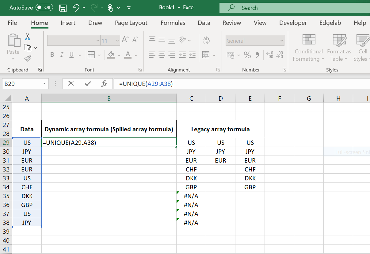
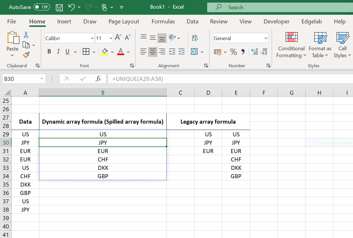
The below image shows that it suffices to type up the function in a cell and press “Enter” to trigger the spill of output on the bordering cells. The right amount of cells is automatically deduced by Excel (second picture for the result).

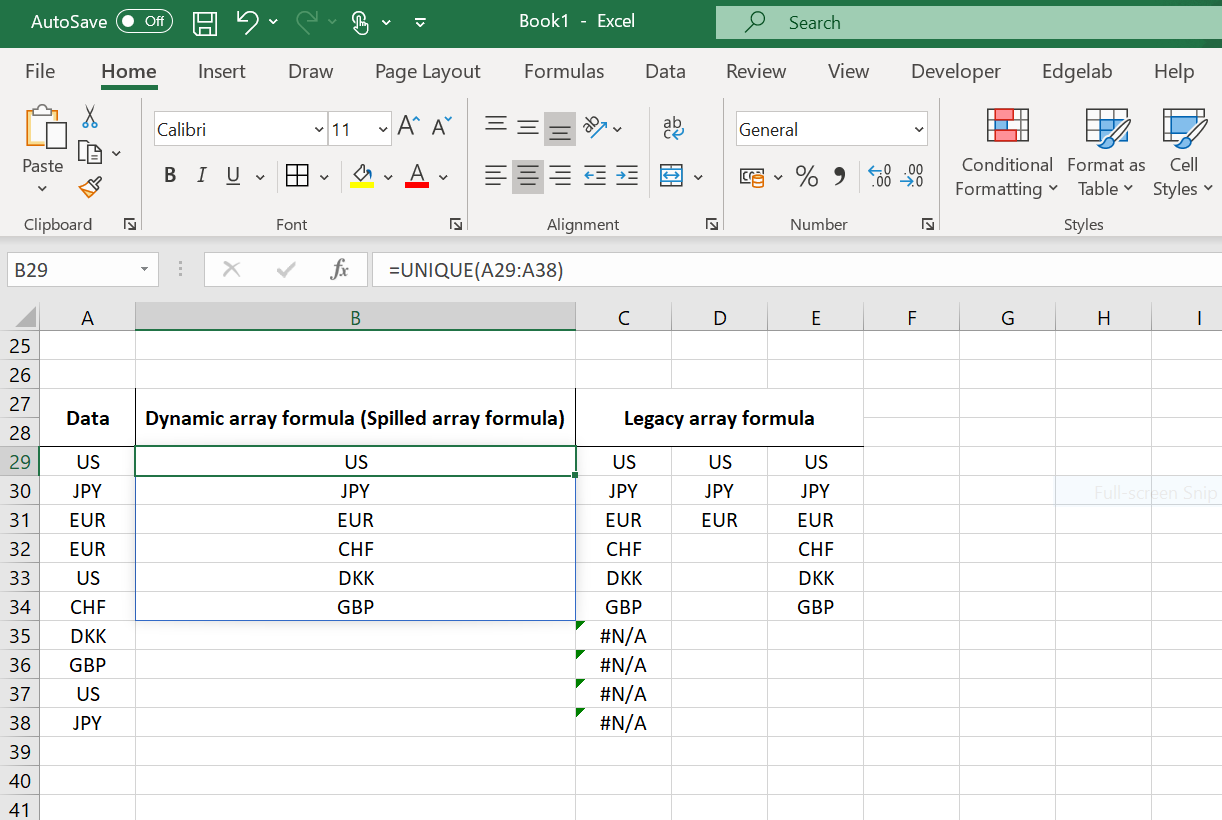
In column B, you have the output of a Spilled array formula. It has a blue frame. Except for the top cell, the rest of the cells are ghosted. If you want to modify something then it has to occur in the cell where the spill comes from (top cell). The changes will spread over the rest of the bordering cells.

In columns C, D, and E, we find the Legacy array formulas where the number of cells over which the results ought to be displayed must be selected before typing the function in the top cell and press Ctrl + Shift + Enter. You can see that in C, the pre-selected area was too long. As a result, Excel filled up the extra cells with #N/A values. In D, the selected area was too short and so only a few cells display the desired output of the function. Finally, in E, the right display of results is achieved as the right amount of pre-selected cells was made. As you may have understood, with Spilled array Formula, only “Enter” needs to be pressed which triggers the automatic spill.