Latest version
Table of content
Edgelab Functions
UDFs listing
- ELASSETCURRENCY
- ELASSETMEASURE
- ELASSETMEASUREPORTFOLIO
- ELASSETNAME
- ELASSETPROXY
- ELBENCHMARKMEASURE
- ELCURRENCIES
- ELCURRENTMEASURE
- ELCURRENTNPV
- ELCUSTOMSTRESSSCENARIO
- ELDISTRIBUTION
- ELDIVERSIFICATIONBENEFIT
- ELENUMEXPOSURETYPES
- ELFIXEDINCOMESHIFT
- ELMARKETDATA
- ELPERFORMANCEMEASURE
- ELPORTWEIGHTTOQUANTITY
- ELPRC
- ELPRC
- ELPRCMETHODOLOGY
- ELPRG
- ELPRGMETHODOLOGY
- ELPROXYCLEANQUANTITIES
- ELRISKFACTOREXPOSUREAGGREGATE
- ELRISKFACTOREXPOSUREFULL
- ELRISKMEASURE
- ELRISKMEASURETAXONS
- ELSTRESSDRIVER
- ELSTRESSDRIVERIDS
- ELSTRESSSCENARIO
- ELSTRESSSCENARIOIDS
- ELVALUATIONDATES
- ELYIELDSOLVING
UDFs details
Last modified in version : 20.7.2
Purpose : retrieve the underlying currency of the instrument
Summary
The elAssetCurrency function retrieves the trading currency of the instrument as saved in the EdgeLab database. This function can also be used as a parameter inside other UDFs (see example below).
Examples
=ELASSETCURRENCY("US0378331005")
Retrieves the currency for the Apple share.
=ELASSETCURRENCY(A10)
Retrieves the currency for the identifier in a cell.
=ELASSETCURRENCY(B2:B10)
Retrieves the currencies for a list of cells.
=ELCURRENTNPV("US0378331005",ELASSETCURRENCY(B2))
Retrieves the NPV of “US0378331005” using ELASSETCURRENCY as one of its parameter.
Syntax
ELASSETCURRENCY(assetIds[])
| Argument name | Description |
|---|---|
| assetIds | Single or multiple asset identifiers (ISIN, FIGI, currency ISO, Edgelab ID). |
Last modified in version : 24.7
Purpose : retrieve risk measures specific to fixed income and structured product instruments
Summary
The ELASSETMEASURE function retrieves a number of different measures such as the probability of hitting the barrier, the yield-to-call, the probability of autocall on the next observation etc. Note: The expected-time-to-maturity measure is only applicable to structured products.
Examples
=ELASSETMEASURE("ytm", **C11:C50**)
Retrieves the yield-to-maturity for each bond in the range C11:C50.
Syntax
ELASSETMEASURE(assetMeasure, assetIds[], isNormalized)
| Argument name | Default | Description |
|---|---|---|
| assetMeasure | The name of the measure to be returned. | |
| assetIds | Single or multiple asset identifiers (ISIN, FIGI, currency ISO, Edgelab ID). | |
| isNormalized (Optional) | False | True: the fund’s asset class’ weights are renormalized, False, the fund asset class’ weights are not |
Last modified in version : -
Purpose : retrieve risk measures specific to fixed income and structured product instruments
Summary
The ELASSETMEASURE function retrieves yields aggregated at the portfolio or asset class level
Examples
=ELASSETMEASUREPORTFOLIO("yield-to-worst", **C11:C50**, **D11:D50**)
Retrieves the yield-to-worst of a portfolio whose instruments are located in C11:C50 with D11:D50 as weights.
Syntax
ELASSETMEASUREPORTFOLIO(assetMeasure, assetIds[], amounts[] isNormalized)
| Argument name | Default | Description |
|---|---|---|
| assetMeasure | The name of the measure to be returned. | |
| assetIds | Single or multiple asset identifiers (ISIN, FIGI, currency ISO, Edgelab ID). | |
| amounts | weights (summing to 100%) | |
| isNormalized (Optional) | False | True: the fund’s asset class’ weights are renormalized, False, the fund asset class’ weights are not |
Last modified in version : 19.04
Purpose : retrieve the name of the instrument
Summary
The ELASSETNAME function retrieves the name of the instrument as saved in the EdgeLab database.
Examples
=ELASSETNAME("US0378331005")
Retrieves the name for an Apple share.
=ELASSETNAME(A1)
Retrieves the name for the identifier in a cell.
=ELASSETNAME(B2:B10)
Retrieves the names for a list of cells.
=ELASSETNAME(B2:B10,30)
Retrieves the names for a list of cells limiting the results to a maximum length of 30 characters.
Syntax
ELASSETNAME(assetIds[], length)
| Argument name | Description |
|---|---|
| assetIds | Single or multiple asset identifiers (ISIN, FIGI, currency ISO, Edgelab ID). |
| length (Optional) | The maximum length above which the returned name will be cropped. The default is to return the full name. |
Last modified in version : -
Purpose : returns the proxy ID if the input asset is replaced by a proxy
Summary
The ELASSETPROXY function indicates the proxy ID if the asset is being replaced by a proxy.
Examples
=ELASSETPROXY("US0378331005")
Retrieves the proxy ID of asset “US0378331005”. The proxy ID is stored in the asset proxy configuration file. It returns a blank cell if the input is not replaced by a proxy.
Syntax
ELASSETPROXY(assetIds)
| Argument name | Description |
|---|---|
| assetIds | Single or multiple asset identifiers (ISIN, FIGI, currency ISO, Edgelab ID). |
Last modified in version : 24.7
Purpose : generic function to retrieve benchmark measures
Summary
The ELBENCHMARKMEASURE function allows retrieving benchmark measures. Currently, the tracking-error, beta, l2-distance and correlation are available. The benchmark can be composed of one position (e.g. an Index) or multiple ones (e.g. a portfolio benchmark). You can specify the amounts in weights or quantities. Bear in mind that if the amount scheme “weight” is selected, the sum of the weights must be equal to 1.
Examples
=ELBENCHMARKMEASURE("tracking-error", "portfolio", C11:C20, B11:B20, "weight", D9, 1, "weight", "CHF", 10, "historicalInnovations")
This function retrieves the tracking error of a portfolio whose assets are in C11:C20 and weights in B11:B20. The benchmark is one position in D9 and could be an Index for example. The amount scheme for the benchmark is “weight” but it could have been “quantity”. The amount is 1 as the benchmark is one position. Then you have the portfolio currency (“CHF” in this example), the time horizon (10 days), and finally the scenario type “historicalInnovation”.
=ELBENCHMARKMEASURE("tracking-error", "contributions", C11:C20, B11:B20, "quantity", D9:D18, E9:E18, "weight", "CHF", 10, "historicalInnovations")
This function retrieves the contributions of the positions to the tracking error between a portfolio and a benchmark. The benchmark is a portfolio whose instruments are in D9:D18. The amount scheme for the benchmark is “weight”. In E9:E18, the weights must sum up to 1. Then, you have the portfolio currency (“CHF” in this example), the time horizon (10 days), and finally the scenario type “historicalInnovation”.
=ELBENCHMARKMEASURE("correlation", "portfolio", C11:C20, B11:B20, "quantity", D9:D18, F9:F18, "quantity", "CHF", 10, "historicalInnovations")
This function retrieves the correlation of a portfolio whose assets are in C11:C20 and quantities in B11:B20. The benchmark is a portfolio whose instruments are in D9:D18. The amount scheme for the benchmark is “quantity”. F9:F18 represents the quantities. Then, you have the portfolio currency (“CHF” in this example), the time horizon (10 days), and finally the scenario type “historicalInnovation”.
Syntax
ELBENCHMARKMEASURE(measure, granularity, assetIds[], amounts[], amountScheme, benchmarkAssetids[], benchmarkAmounts[], benchmarkAmountScheme, currency, riskHorizon, scenarioType, annualized, scalingHorizon, liquidityAdjusted)
| Argument name | Default | Description |
|---|---|---|
| measure | The name of the measure to be returned. | |
| granularity | portfolio or contributions (only works for tracking-error and l2-distance) | |
| assetIds | Single or multiple asset identifiers (ISIN, FIGI, currency ISO, Edgelab ID). | |
| amounts | 1 (for quantitites) | quantities or weights of the assets. Weights must sum up to 100%. |
| amountScheme (Optional) | quantity | quantity or weight |
| benchmarkAssetids | Single or multiple asset identifiers (ISIN, FIGI, currency ISO, Edgelab ID). | |
| benchmarkAmounts | 1 (for quantitites) | quantities or weights of the assets. Weights must sum up to 100%. |
| benchmarkAmountScheme (Optional) | quantity | quantity or weight |
| currency | The ISO code of the reference currency for deriving the calculation results. Specify “local” to use the instruments native currency where appropriate. It is mandatory to specify a currency when the granularity is “portfolio”. | |
| riskHorizon (Optional) | 10 | The time interval over which the risks are estimated (i.e. between now and now + risk-horizon). |
| scenarioType (Optional) | historicalInnovations | How the possible scenarios for the asset prices are computed. |
| annualized (Optional) | FALSE | Whether the result should be expressed as an annualized figure. True or False. |
| scalingHorizon (Optional) | RiskHorizon | |
| liquidityAdjusted (Optional) | FALSE | If true, then risk computations will account for the liquidity risk. |
Last modified in version : -
Purpose : retrieve the supported currency supported by Edgelab.
Summary
This functions exposes the supported currency that are in Edgelab database.
Examples
=ELCURRENCIES()
Exposes a list of currency that Edgelab supports.
Syntax
ELCURRENCIES()
Last modified in version : -
Purpose : generic function to retrieve specific measures
Summary
The ELCURRENTMEASURE function retrieves a number of different current measures for a list of instruments. The function supports positions, contributions and portfolio as calculation levels.
Examples
In these examples the risk measure that the function aims to retrieve is the net present value (NPV).
=ELCURRENTMEASURE("NPV","positions",C11,D11,"quantity","EUR", "relative")
Retrieves the current NPV of one unique asset whose ID is in cell C11 and quantity in cell D11. The currency is EUR. measureType is set to relative.
=ELCURRENTMEASURE("NPV","portfolio",C11:C50,D11:D50,"quantity","EUR", "relative")
Retrieves the current NPV of a portfolio where C11:C50 are the asset IDs within the portfolio and D11:D50 are the quantities of each asset. The currency is EUR.
=ELCURRENTMEASURE("NPV","portfolio",{"CHF","EUR"},{1000,1000},"quantity", "EUR", "relative")
This example can be copied and pasted to Excel and will give an instantaneous result.
Syntax
ELCURRENTMEASURE(currentMeasure, granularity, assetIds[], amounts[], amountScheme, currency, measureType)
| Argument name | Default | Description |
|---|---|---|
| currentMeasure | The name of the measure to be returned. | |
| granularity | The granularity at which the results should be calculated (individual asset, portfolio). | |
| assetIds | Single or multiple asset identifiers (ISIN, FIGI, currency ISO, Edgelab ID). | |
| amounts | 1 (for quantitites) | quantities or weights of the assets. Weights must sum up to 100%. |
| amountScheme (Optional) | quantity | quantity or weight |
| currency | local | The ISO code of the reference currency for deriving the calculation results. Specify “local” to use the instruments native currency where appropriate. It is mandatory to specify a currency when the granularity is “portfolio”. |
| measureType (Optional) | relative | Whether the result should be normalized. The input should be “relative” or “absolute”. “True” or “False” are still supported for the moment. |
Last modified in version : 20.04
Purpose : retrieve the current valuation of the product
Summary
The ELCURRENTNPV function retrieves the current valuation (Edgelab valuation) as saved in the Edgelab database.
Examples
=ELCURRENTNPV("US0378331005")
Retrieves the price of an Apple share.
=ELCURRENTNPV(A10)
Retrieves the price for the identifier in a cell.
=ELCURRENTNPV("US0378331005", "CHF")
Retrieves the price of an Apple share converted to Swiss Francs.
Syntax
ELCURRENTNPV(assetIds[], currency)
| Argument name | Description |
|---|---|
| assetIds | A single asset identifier representing the instrument (ISIN, FIGI, currency ISO, Edgelab ID). |
| currency | The ISO code of the reference currency for deriving the calculation results. Specify “local” to use the instruments native currency where appropriate. It is mandatory to specify a currency when the granularity is “portfolio”. |
Last modified in version : -
Purpose : retrieve the profit and loss of a portfolio or its instruments given a list of shock on a stress driver
Summary
After having defined a shock amplitude for each stress driver, the ELCUSTOMSTRESSSCENARIO function retrieves on demand the profit and loss of a portfolio. This function supports only positions and portfolio as calculation levels.
This function can be used instead of the pre-defined macro stress scenarios and =ELSTRESSDRIVER(). Indeed, it offers more reliable estimates and more customization.
The constraints:
- 50 custom stress scenarios per organization;
- Maximum 3 stress drivers per custom scenario;
- If the scenario hasn’t been used in 10 days, it is no longer precomputed during our night run.
If you reach the limit on the number of custom stress scenarios per organisation and you would like to test new stress tests, please contact our support through our Edgelab support portal so that they can set the count back to 0.
Examples
=ELCUSTOMSTRESSSCENARIO("pnl","portfolio",D5:D7,E5:E7,F5:F7,G5:G7,H5:H7,"quantity","CHF","relative")
Calculates the P&L impact an interest curve stress would have on a portfolio of instruments defined in column C (with corresponding quantities in column D) expressed in CHF.
Syntax
ELCUSTOMSTRESSSCENARIO(measure,granularity, driverIds[], shockTypes[], shockValues[], assetsIds[], amounts[], amountScheme, currency, measureType)
| Argument name | Default | Description |
|---|---|---|
| measure | “pnl” (Profit and Loss). | |
| granularity | The granularity at which the results should be calculated (individual asset, portfolio). | |
| driverIds | The IDs of a pre-defined scenario to serve as the basis for the simulation. | |
| shockTypes | relative | relative or absolute (Check the stress scenarios dedicated tables) |
| shockValues | any number | |
| assetsIds | Single or multiple asset identifiers (ISIN, FIGI, currency ISO, Edgelab ID). | |
| amounts | 1 (for quantitites) | quantities or weights of the assets. Weights must sum up to 100%. |
| amountScheme (Optional) | quantity | quantity or weight |
| currency | local | The ISO code of the reference currency for deriving the calculation results. Specify “local” to use the instruments native currency where appropriate. It is mandatory to specify a currency when the granularity is “portfolio”. |
| measureType (Optional) | relative | Whether the result should be normalized. The input should be “relative” or “absolute”. “True” or “False” are still supported for the moment. |
Last modified in version : -
Purpose : retrieve the forecasted scenarios of a portfolio or an instrument
Summary
The ELDISTRIBUTION function retrieves the forecasted scenarios of a portfolio or an instrument.
Examples
=ELDISTRIBUTION("pnl","positions", C11,D11,"quantity","EUR", 252, "historicalInnovations", "relative", FALSE)
Spans the distribution of asset C11 using the historical innovation model with a time horizon of 252 days. The quantity is in cell D11. The currency is EUR. The last parameter is set to FALSE hence the output will be a column (a row otherwise).
=ELDISTRIBUTION("pnl","portfolio",{"CHF","EUR"}, {1000,1000},"quantity","EUR", 252,"historicalInnovations", "relative", FALSE)
This example can be copied and pasted to Excel and will give an instantaneous result.
Syntax
ELDISTRIBUTION(measure, granularity, assetsIds[], amounts[], amountScheme, currency, riskHorizon, scenarioType, measureType, isRow)
| Argument name | Default | Description |
|---|---|---|
| measure | “pnl” (Profit and Loss). | |
| granularity | The granularity at which the results should be calculated (individual asset, portfolio). | |
| assetsIds | Single or multiple asset identifiers (ISIN, FIGI, currency ISO, Edgelab ID). | |
| amounts | quantities or weights of the assets. Weights must sum up to 100%. | |
| amountScheme (optional) | quantity | quantity or weight |
| currency | local | The ISO code of the reference currency for deriving the calculation results. Specify “local” to use the instruments native currency where appropriate. It is mandatory to specify a currency when the granularity is “portfolio”. |
| riskHorizon (Optional) | 10 | The time interval over which the risks are estimated (i.e. between now and now + risk-horizon). |
| scenarioType (Optional) | historicalInnovations | How the possible scenarios for the asset prices are computed. |
| measureType (Optional) | relative | Whether the result should be normalized. The input should be “relative” or “absolute”. “True” or “False” are still supported for the moment. |
| isRow (Optional) | false | If sets to true, the output is displayed as a row. |
Last modified in version : -
Purpose : measure the diversification benefit in a portfolio
Summary
With ELDIVERSIFICATIONBENEFIT, you can measure how much your portfolio benefits from diversification. The Add-in function can be translated as such:
The numerator is the risk measure of the portfolio. The denominator is the sum of the risk measures of each position, weighted by the position’s weights.
The larger is the diversification benefit, the more the portfolio benefits from diversification. The risk measure can be either volatility, value-at-risk, or expected shortfall.
Intuitively, if there is no diversification in the portfolio, all the positions behave in the same way and the correlation between positions are 1. Then, the risk measure of the portfolio is equal to the risk measure of the positions, the fraction is equal to 1 and there is no diversification benefit. For the diversification benefit to increase, the positions in the portfolio should have a small correlation so that the portfolio risk is smaller than the total risk of the positions.
A simple example with risk measured by the volatility and constant correlation
Consider a simple example with a portfolio made of $n$ positions, all with the same weights $w_i = 1/n$ and the same volatility $\sigma$. All the positions share the same correlation $\rho$, namely the correlation between 2 positions $i$ and $j$ is $\rho_{i,j} = \rho$ (and the correlation is one when $i = j$). The risk measure is the volatility.
With this setting, the analytical computations are straightforward.
At the position level, the risk of each position is $\sigma$, and the total risk evaluated at the position level is $\sum_{i} w_{i} \sigma = \sigma$.
At the portfolio level, the risk is given by
\[\sigma(portfolio) = \sigma \sqrt{\rho + (1-\rho)/n}.\]The ratio of the risks at portfolio and position levels is not depending on $\sigma$, but only on the correlation and the number of positions. The diversification benefit is $DB = 1 - \sqrt{\rho + (1-\rho)/n}$. If the correlation is one, \(\rho = 1\), diversification is not possible as all assets behave similarly. In this case, the diversification benefit is zero, namely regardless of the number of positions, diversification cannot be achieved.
If the correlation is zero, the diversification benefit is $DB = 1 - \sqrt{1/n}$, namely the larger is the portfolio, the larger the diversification benefit.
The correlation can be negative. For 2 random variables, the correlation is between -1 and +1. But with more random variables, the correlations cannot be all -1 for all pairs of variables! For the present model with a constant correlation coefficient, it can be shown that the correlation coefficient is bounded with
\[\frac{1}{n-1} \leq \rho \leq 1\]With the correlation at the lower bound, the volatility of the portfolio is null, and the diversification benefit is 1. This is the best that can be achieved. Alas, it is very difficult to find many assets with mutual correlation coefficients that are all negatives. Hence, this case is rather theoretical, and the realistic domain for this model is to consider positive correlations $\rho$.
For a correlation between 0 and 1, the term in $\rho$ in the square root is the component that cannot be diversified away. The second term given by $(1-\rho)/n$ is the part that is decreasing with increasing portfolio size. This simple model concludes that to have the largest diversification benefit, a portfolio should be constructed from a large number of positions with a low correlation $\rho$.
This simple model was constructed to make straightforward analytical computations. In general, the correlations on a typical stock market are in the range of 10 to 60%, and rarely null or negative. Then, the volatilities differ, and the position weights are different. But the conclusions of the simple model remain, namely diversified portfolios are made of a large number of positions with low correlations. And completely diversified portfolios cannot be constructed in practice, even with a very large number of positions.
Examples
=ELDIVERSIFICATIONBENEFIT("volatility", C11:C50, D11:D50, "quantity", "EUR", 10, 0.95, "historicalInnovations", True)
The above example would return the diversification benefit for the volatility of a portfolio whose assets and quantities are in C11:C50 and D11:D50 respectively. The portfolio currency is EUR and the scenario type is historicalInnovation. The rest of the parameters are the default ones.
Syntax
ELDIVERSIFICATIONBENEFIT(riskMeasure, assetsIds[], amounts[], amountScheme, prices[], currency, riskHorizon, confidenceLevel, scenarioType, annualized, scalingHorizon)
| Argument name | Default | Description |
|---|---|---|
| riskMeasure | The name of the measure to be returned. | |
| assetsIds | Single or multiple asset identifiers (ISIN, FIGI, currency ISO, Edgelab ID). | |
| amounts | 1 (for quantitites) | quantities or weights of the assets. Weights must sum up to 100%. |
| amountScheme (Optional) | quantity | quantity or weight |
| currency | local | The ISO code of the reference currency for deriving the calculation results. Specify “local” to use the instruments native currency where appropriate. It is mandatory to specify a currency when the granularity is “portfolio”. |
| prices (Optional) | Edgelab prices | You have the possibility to insert your own instrument prices. This parameter is optional and the function will take the Edgelab prices by default. |
| riskHorizon (Optional) | 10 | The time interval over which the risks are estimated (i.e. between now and now + risk-horizon). |
| confidenceLevel (Optional) | 0.95 | The confidence level for the tail statistics estimators VaR and ES. It is number in percent between 85 and 99 [%]. |
| scenarioType (Optional) | historicalInnovations | How the possible scenarios for the asset prices are computed. |
| annualized (Optional) | true | Whether the result should be expressed as an annualized figure. True or False. |
| scalingHorizon (Optional) | RiskHorizon |
Last modified in version : -
Purpose : retrieve the list of the risk factor buckets.
Summary
The ELENUMEXPOSURETYPES returns simply the list of the exposures that constitute the source of risk of an asset. The function has no parameters. When the function is called, 5 risk factors are displayed: RiskFreeZCBonds, RiskyZCBonds, Underlyings - spot, Underlyings - implied volatility, Cash.
Syntax
ELENUMEXPOSURETYPES()
Last modified in version : 20.7
Purpose : calculate aggregate risk sensitivity
Summary
This function calculates a high level aggregate sensitivity figure of a fixed income asset. It takes into account shifts in both interest rate and credit curves by combining the effects of several standard sensitivity measures.
Formula
Examples
=ELFIXEDINCOMESHIFT(A1,B1) or =ELFIXEDINCOMESHIFT(100,3047)
Returns the sensitivity based solely on the assets DV01 (second argument) and the assumed shift in interest rates (first argument).
=ELFIXEDINCOMESHIFT(A1,B1,C1) or =ELFIXEDINCOMESHIFT(100,3047,9205)
Returns the sensitivity taking into account, in addition to the precedent function, the instruments convexity (third argument) with regards to interest rate changes.
=ELFIXEDINCOMESHIFT(A1,B1,C1,D1,E1) or =ELFIXEDINCOMESHIFT(100,3047,9205,100,-2993)
Returns the sensitivity including, in addition to the precedent function, the instruments sensitivity to credit curve shifts (CS01) (fifth argument) and the corresponding assumed shift in the curve (fourth argument).
Syntax
ELFIXEDINCOMESHIFT(irShift, dv01, convexity, creditShift, cs01)
| Argument name | Description |
|---|---|
| irShift | The assumed parallel shift in interest rates expressed in basis points (bps). |
| dv01 | The DV01 of the asset: its sensitivity to 1 bp change in interest rates. |
| convexity (Optional) | The convexity of the asset: measures the non-linearity of the asset interest rate sensitivity. |
| creditShift (Optional) | The assumed parallel shift in the asset credit curves expressed in basis points (bps). |
| cs01 (Optional) | The CS01 of the asset: its sensitivity to 1 bp change in the credit curve. |
Last modified in version : -
Purpose : retrieve the parameter of the specified instrument
Summary
The ELMARKETDATA function retrieves the specific parameter of the instrument as saved in the EdgeLab database.
Examples
=ELMARKETDATA("US0378331005", "liquidityHorizon")
Retrieves the liquidity horizon for an Apple share.
Syntax
ELMARKETDATA(assetsIds[], parameterName)
| Argument name | Description |
|---|---|
| assetsIds | Single or multiple asset identifiers (ISIN, FIGI, currency ISO, Edgelab ID). |
| parameterName | “liquidityHorizon” |
Last modified in version : -
Purpose : generic function to retrieve performance measures
Summary
The ELPERFORMANCEMEASURE function retrieves performance measures based on methods like capital market assumptions. Make sure your have provided our client success team with the mapping between instruments and CMAs and the necessaty inputs like the expected returns and covariance matrix.
Examples
In these examples the risk measure that the function aims to retrieve is the value at risk (VaR).
=ELPERFORMANCEMEASURE("expected-return","positions",C11,D11,"weight","EUR", "market-assumptions","relative")
Retrieves the expected return of the positions based on their capital market assumptions.
=ELPERFORMANCEMEASURE("sharpe-ratio","portfolio",C11,D11,"weight","USD", "market-assumptions","relative")
Retrieves the Sharpe Ratio of the portfolio based on their capital market assumptions.
Syntax
ELPERFORMANCE(measure, granularity, assetIds[], amounts[], amountScheme, currency, methodType, measureType)
| Argument name | Default | Description |
|---|---|---|
| measure | The name of the measure to be returned. | |
| granularity | portfolio or positions | |
| assetIds | Single or multiple asset identifiers (ISIN, FIGI, currency ISO, Edgelab ID). | |
| amounts | 1 (for quantitites) | quantities or weights of the assets. Weights must sum up to 100%. |
| amountScheme (Optional) | quantity | quantity or weight |
| currency | local | The ISO code of the reference currency for deriving the calculation results. Specify “local” to use the instruments native currency where appropriate. It is mandatory to specify a currency when the granularity is “portfolio”. |
| methodType (Optional) | market-assumptions | market-assumptions |
| measureType (Optional) | relative | Whether the result should be normalized. The input should be “relative” or “absolute”. “True” or “False” are still supported for the moment. |
Last modified in version : 20.7.2
Purpose : calculate the required quantity of an asset to reach a target weight in a portfolio of a given value
Summary
The ELPORTWEIGHTTOQUANTITY function converts the asset’s weight into quantity given that the instrument is part of a portfolio which has a specific value and currency.
Examples
=ELPORTWEIGHTTOQUANTITY("US0378331005",0.2,"CHF",1000000)
Calculates the number of Apple shares required to achieve a target weight of 20% within a portfolio of 1,000,000 CHF.
=ELPORTWEIGHTTOQUANTITY(A1,30%,"GBP",500000)
Calculates the required quantity of the instrument whose ID is specified in cell A1 to achieve a target weight of 30% within a portfolio of 500,000 GBP.
=ELPORTWEIGHTTOQUANTITY(A1:A25,B1:B25,"GBP",500000)
The function is now dynamic. In this example, it calculates the required quantities of the instruments (A1:A25) to achieve their respected weights (B1:B25) within a portfolio of 500,000 GBP.
Syntax
ELPORTWEIGHTTOQUANTITY(assetsIds[], weights[], portfolioCurrency, portfolioValue)
| Argument name | Description |
|---|---|
| assetsIds | A single asset identifier representing the instrument (ISIN, FIGI, currency ISO, Edgelab ID). |
| weights | The desired weight of the instrument expressed in percentage within the portfolio. |
| portfolioCurrency | The ISO code of the currency in which the overall portfolio value is specified. |
| portfolioValue | The total value of the portfolio within which the desired weight should be achieved. |
Last modified in version : 21.3
Purpose : the Product Risk Classification (PRC) of instruments
Summary
The ELPRC function provides you with the PRC of a single or a range of assets.
Examples
=ELPRC("US0378331005")
Retrieves the PRC of an Apple share using the default methodology.
=ELPRC(A2:A10, "2020q3")
Retrieves the PRC for a list of assets using the methodology “historicalInnovations”.
Syntax
ELPRC(assetIds[], methodology)
| Argument name | Default | Description |
|---|---|---|
| assetIds | Single or multiple asset identifiers (ISIN, FIGI, currency ISO, Edgelab ID). | |
| methodology | 2020q3 | “2020q3” or “2020q3-liquidity” |
Last modified in version : 12.12
Purpose : the Product Risk Classification (PRC3) of instruments
Summary
The ELPRC3 function provides you with the PRC of a single or a range of assets. the PRC can be based either on the global or asia methodology. The grade includes a market, credit and liquidity risk portion which can be displayed.
Examples
=ELPRC3("US0378331005")
Retrieves the adjusted PRC of an Apple share using the default methodology which is the global one.
=ELPRC3(A2:A10, "global")
Retrieves the adjusted PRC for a list of assets using the methodology “global”.
=ELPRC3("US0378331005", "asia", {"raw", "stabilized", "adjusted"}, "TRUE", "TRUE", "TRUE")
Retrieves the raw, stabilized and adjusted PRCs for an Apple share using the ‘asia’ methodology, displaying the model used to compute the grade, along with the PRC decomposition into market, credit, and liquidity risk buckets and their corresponding weights.
| US0378331005 | Raw | Stabilized | Adjusted | Market prc | Liquidity prc | Credit prc | Market weight | Liquidity weight | Credit weight | Model |
|---|---|---|---|---|---|---|---|---|---|---|
| 3.24027 | 3 | 3 | 5.00994 | 1.00614 | 1.53184 | 0.53483 | 0.28872 | 0.17643 | computed |
Syntax
ELPRC3(assetIds[], methodology, prc[], components, model, headers)
| Argument name | Default | Description |
|---|---|---|
| assetIds | Single or multiple asset identifiers (ISIN, FIGI, currency ISO, Edgelab ID). | |
| methodology | global | Optional field defining the methodology to be used for risk classification, can be “global” or “asia” |
| prc | adjusted | Optional field defining the PRC value to return, can be “raw”, “stabilized” or “adjusted”. The “raw” PRC corresponds to the weighted sum of market, credit and liquidity grades. |
| components | FALSE | Optional field showing the details of the PRC composition, can be “FALSE” or “TRUE” |
| model | FALSE | Optional field showing the model used to compute the adjusted PRC, can be “FALSE” or “TRUE” |
| headers | FALSE | Optional field showing the header of the response can be “FALSE” or “TRUE” |
To benefit from this feature please contact our sales representatives by sending an email to sales@evooq.ch.
Last modified in version : -
Purpose : retrieve the parameters and intervals based on which the PRC levels are defined.
Summary
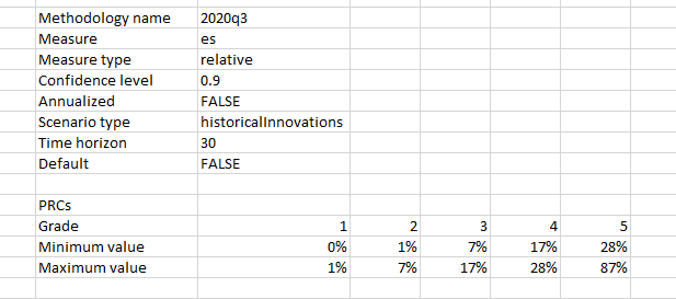
The ELPRCMETHODOLOGY function returns 3 types of output. If no parameters are inserted, the output will be the Edgelab methodologies that can be inserted as the first parameter: “2020q3” and “2020q3-liquidity”. If only “MethodologyName” is specified, you’ll get the summarized view, namely a table with the PRC levels and their intervals (maximum and minimum value) - the value is the relative ES. Finally, if you set to TRUE “ShowDetails”, in addition to the PRC levels and values, you’ll have a view of the different parameters used during the calibration (e.g. confidence level, time horizon, etc).
Examples
=ELPRCMETHODOLOGY("2020q3", TRUE)
Retrieves the parameters used in the PRC calibration and the intervals provided by the distribution of relative ES. The distribution comes from a universe of 11000 assets that represent the market. For more details, do not hesitate to ask for the PRC_PRG_methodology documentation. The parameters are the risk methodology, the risk measure, the measure type (relative or absolute), the confidence level, annualized, the scenario type (“historicalInnovations” or “historicalReturns”), the time horizon, and default. If default is FALSE, then the selected methodology in “MethodologyName” is not the default methodology, or else it is.
Syntax
ELPRCMETHODOLOGY(methodologyName, showDetails)
| Argument name | Description | |
|---|---|---|
| methodologyName | “2020q3” or “2020q3-liquidity” | |
| showDetails (Optional) | FALSE | Boolean, if set to TRUE, the parameters used in the calibration are shown, or else only the PRC levels and the intervals are displayed. |
Last modified in version : 18.12
Purpose : retrieve the Portfolio Risk Grade (PRG) of a portfolio
Summary
The ELPRG function returns the Portfolio Risk Grade of a portfolio in a reference currency. This function supports only contributions and portfolio as calculation levels.
Examples
=ELPRG("portfolio",C11:C50,D11:D50,"quantity","EUR")
Retrieves the risk grade of a portfolio of EUR instruments with the list of instruments provided in column C and their corresponding quantities in column D.
=ELPRG("contributions",C11:C50,D11:D50, "weight","EUR")
Retrieves the contributions of each instrument (column C) to the portfolio (EUR) PRG. Their corresponding weights are in column D.
Syntax
ELPRG(granularity, assetIds[], amounts[], amountScheme, currency, isSimulation)
| Argument name | Description | ||
|---|---|---|---|
| granularity | granularity | The granularity at which the results should be calculated (individual asset, portfolio). | |
| assetIds | Single or multiple asset identifiers (ISIN, FIGI, currency ISO, Edgelab ID). | ||
| amounts | 1 (for quantitites) | quantities or weights of the assets. Weights must sum up to 100%. | |
| amountScheme (Optional) | quantity | quantity or weight | |
| currency | The ISO code of the reference currency for deriving the calculation results. Specify “local” to use the instruments native currency where appropriate. It is mandatory to specify a currency when the granularity is “portfolio”. | ||
| isSimulation (Optional) | False | Boolean, if set to True, the calibration is flagged as a simulation and does not impact the portfolio’s PRGs running in production. If it is set to False the calibration is the one in production. |
Last modified in version : -
Purpose : retrieve the parameters and bounds to which each portfolio models have been calibrated upon.
Summary
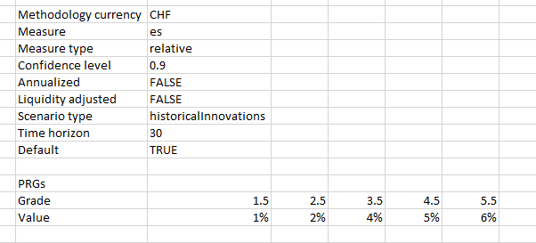
The ELPRGMETHODOLOGY function returns 3 types of output. If no parameters are inserted, the output will be the currencies upon which your portfolio models are calibrated. If only “MethodologyCurrency” is specified, you’ll get the summarized view, namely a table with the PRG levels and their bounds (“Value”). Finally, if you set to TRUE “ShowDetails”, in addition to the PRG levels and values, you’ll have a view on the different parameters used during the calibration (e.g. confidence level, time horizon etc.) The simulation parameter retrieves the bounds of the simulated strategies if set to True. While having strategies in production, you may want to test out new allocations or positions to simulate the impact on your clients’ portfolios. To calibrate your PRG bounds, do not hestitate to use our PRG administrator portal. Feel free to contact our client success team for further information: client.delivery@edgelab.ch.
Example
=ELPRGMETHODOLOGY("USD", TRUE, FALSE)
Retrieves the parameters used in the PRG calibration and the bounds of the portfolio models. The parameters are the currency, the risk measure, the measure type (relative or absolute) the confidence level, annualized, liquidity adjusted, the scenario type (“historicalInnovations” or “historicalReturns”), the time horizon and default. If default is FALSE, then the currency inserted in “MethodologyCurrency” is not the fallback currency, or else it is. A fallback currency is unique and is the reference currency for any portfolio that is based on a currency that is not part of the PRG calibration. The parameter liquidity adjusted is boolean. If it is True, it means the PRG calibration and computation account for the liquidity risk of the portfolio’s positions.
Syntax
ELPRGMETHODOLOGY(methodologyCurrency, showDetails, isSimulation)
| Argument name | Description | |
|---|---|---|
| methodologyCurrency | Any currency that has been used in the calibration. Type =ELPRGMETHODOLOGY() in a cell to see the list of available currencies. |
|
| showDetails (Optional) | False | Boolean, if set to True, the parameters used in the calibration are shown, or else only the PRG levels and bounds are displayed. |
| isSimulation (Optional) | False | Boolean, if set to True, the calibration is flagged as a simulation and does not impact the portfolio’s PRGs running in production. If it is set to False the calibration is the one in production. |
Last modified in version : 19.04
Purpose : return a cleaned quantity between a main quantity and a proxy quantity.
Summary
The function ELPROXYCLEANQUANTITIES is a help function, which provides a simplified way to handle quantities. This functions also checks for null or empty strings.
Examples
=ELPROXYCLEANQUANTITIES(A1) or =ELPROXYCLEANQUANTITIES(A1, "")
Returns a verified version of the quantity in A1. If the value referenced in the second parameters is empty or null, this value is discarded.
=ELPROXYCLEANQUANTITIES(A1, B2)
In this case, the function overrides the quantity in A1 and returns a checked version of the quantity in B2. This allows an override of the quantity in A1, for example in the case where a proxy asset is used.
Syntax
ELPROXYCLEANQUANTITIES(quantityMain, quantityOverride)
| Argument name | Description |
|---|---|
| quantityMain | A main quantity. |
| quantityOverride | A replacement quantity. |
Last modified in version : -
Purpose : retrieve the risk factor values (aggregated by group of risk factors) impacting the valuation of the position
Summary
The ELRISKFACTOREXPOSUREAGGREGATE function displays the value (aggregated) of each of the risk factor buckets namely - RiskFreeZCBonds, RiskyZCBonds, Underlyings, Cash. The sum of these values equals 1 which is the normalized valuation of the position’s value. These exposures result from the breakdown that is the equivalent valuation of a position into its risk factors (sources of risk). RiskFreeZCBonds and RiskyZCBonds reflect the interest rate and issuer’s risky rate dependency while underlyings reflect the dependence on the underlyings’ spots and implied volatilities (in the case of options for instance).
Examples
Let’s take the example of the BRC CH0579768547.
=ELRISKFACTOREXPOSUREAGGREGATE("positions",CH0579768547,1,"CHF",TRUE)
Below is the raw output of calling the above function. Of course the output can be formated.
 In this case, the conclusion is that the main the valuation’s driver are the RiskyZCBonds (the issuer) and the Cash risk factors. It is expected as this BRC has experienced no “barrier-event”.
Syntax
ELRISKFACTOREXPOSUREAGGREGATE(assetIds[], currency, headerRow)
| Argument name | Default | Description |
|---|---|---|
| assetIds | Single or multiple asset identifiers (ISIN, FIGI, currency ISO, Edgelab ID). | |
| currency | The ISO code of the reference currency for deriving the calculation results. Specify “local” to use the instruments native currency where appropriate. It is mandatory to specify a currency when the granularity is “portfolio”. | |
| headerRow (Optional) | FALSE | Boolean. If true, the headers are displayed, if false, they are not. |
Last modified in version : -
Purpose : retrieve the risk factor values impacting the valuation of the position
Summary
The ELRISKFACTOREXPOSUREFULL function displays the value of each of the risk factor buckets namely - RiskFreeZCBonds, RiskyZCBonds, Underlyings - spot, Underlyings - implied volatility, Cash. The output is more granular than ELRISKFACTOREXPOSUREAGGREGATE. The sum of these values equals 1 which is the normalized valuation of the position’s value. These exposures result from the breakdown that is the equivalent valuation of a position into its risk factors (sources of risk). RiskFreeZCBonds and RiskyZCBonds reflect the interest rate and issuer’s risky rate dependency while underlyings reflect the dependence on the underlyings’ spots and implied volatilities (in the case of options for instance).
Examples
Let’s take the example of the BRC CH0579768547.
=ELRISKFACTOREXPOSUREFULL(CH0579768547,"CHF")
Below is the raw output of calling the above function. Of course the output can be formated.
 In this case, the conclusion is that the main the exposure are the RiskyZCBonds (the issuer) and the CHF Cash component displayed in the screenshot. It is expected as this BRC has experienced no “barrier-event”.
Syntax
ELRISKFACTOREXPOSUREFULL(assetId, amount, amountScheme, currency, exposureTypes)
| Argument name | Default | Description |
|---|---|---|
| assetId | A single asset identifier representing the instrument (ISIN, FIGI, currency ISO, Edgelab ID). | |
| currency | The ISO code of the reference currency for deriving the calculation results. Specify “local” to use the instruments native currency where appropriate. It is mandatory to specify a currency when the granularity is “portfolio”. | |
| exposureTypes (Optional) | Return all types of risk factors | RiskFreeZCBonds, RiskyZCBonds, Underlyings - spot, Underlyings - implied volatility, Cash. |
Last modified in version : -
Purpose : generic function to retrieve any type of risk figures
Summary
The ELRISKMEASURE function retrieves a number of different risk measures for a list of instruments based on a variety of scenarios and calculation parameters.
Examples
In these examples the risk measure that the function aims to retrieve is the value at risk (VaR).
=ELRISKMEASURE("var","positions",C11,D11,"weight","EUR", 10, 0.95,,,"historicalInnovations", "relative", TRUE)
Retrieves the value at risk of one unique asset whose ID and weight are is in cell C11 and D11 respectively. The currency is EUR. The RiskHorizon is 10 days, the CondifenceLevel is 95%, the ScenarioType is historical innovation and MeasureType and Annualized are set to “relative” and TRUE. These are the default parameters.
=ELRISKMEASURE("var","portfolio",C11:C50,D11:D50,"quantity","EUR", 10,,0.925,0.975, "historicalInnovations", "relative", TRUE)
Retrieves the value at risk of a portfolio whose positions and quantities are displayed by C11:C50 and D11:D50 respectively. The currency is EUR. Instead of using the confidence level, confidence lower and upper bounds are parametrized to obtain a “meanVaR”. The measure is more robust as more points are taken into account in the computation. For instance, the impact is quite strong when looking at the var contributions.
=ELRISKMEASURE("var","portfolio",{"CHF","EUR"},{0.5, 0.5},"weight","EUR", 10, 0.95,,, "historicalInnovations", "relative", TRUE, 1, TRUE)
This example can be copied and pasted to Excel and will give an instantaneous result. The function computes the portfolio VaR for a risk horizon of one day and accounts for positions’ liquidity risk.
=ELRISKMEASURE("var","contributions",C11:C50,D11:D50, "quantity", "EUR", 10, 0.95,,, "historicalInnovations", "absolute", TRUE, 20, TRUE)
Retrieves the contributions to the portfolio risk of each of the positions for a 20 days risk horizon. C11:C50 stands for the asset IDs of the portfolio and D11:D50 for the quantities. The currency is EUR.
Syntax
ELRISKMEASURE(measure, granularity, assetIds[], amounts[], amountScheme, currency, riskHorizon, confidenceLevel, confidenceLowerBound, confidenceUpperBound, scenarioType, measureType, annualized, scalingHorizon, liquidityAdjusted)
| Argument name | Default | Description |
|---|---|---|
| measure | The name of the measure to be returned. | |
| granularity | The granularity at which the results should be calculated (individual asset, portfolio). | |
| assetIds | Single or multiple asset identifiers (ISIN, FIGI, currency ISO, Edgelab ID). | |
| amounts | 1 (for quantitites) | quantities or weights of the assets. Weights must sum up to 100%. |
| amountScheme (Optional) | quantity | quantity or weight |
| currency | local | The ISO code of the reference currency for deriving the calculation results. Specify “local” to use the instruments native currency where appropriate. It is mandatory to specify a currency when the granularity is “portfolio”. |
| riskHorizon (Optional) | 10 | The time interval over which the risks are estimated (i.e. between now and now + risk-horizon). |
| confidenceLevel (Optional) | 0.95 | The confidence level for the tail statistics estimators VaR and ES. It is number in percent between 85 and 99 [%]. |
| confidenceLowerBound (Optional) | The confidence bounds are to be used with VaR only. They are numbers in percent between 85 and 99 [%]. The VaR is then computed over a range of points (“meanVaR”). | |
| confidenceUpperBound (Optional) | The confidence bounds are to be used with VaR only. They are numbers in percent between 85 and 99 [%]. The VaR is then computed over a range of points (“meanVaR”). | |
| scenarioType (Optional) | historicalInnovations | How the possible scenarios for the asset prices are computed. |
| measureType (Optional) | relative | Whether the result should be normalized. The input should be “relative” or “absolute”. “True” or “False” are still supported for the moment. |
| annualized (Optional) | FALSE | Whether the result should be expressed as an annualized figure. True or False. |
| scalingHorizon (Optional) | RiskHorizon | |
| liquidityAdjusted (Optional) | FALSE | If true, then risk computations will account for the liquidity risk. |
Last modified in version : -
Purpose : generic function to retrieve any type of risk figures at the taxon level
Summary
The ELRISKMEASURETAXONS function retrieves different risk measures for a list of taxons based on a variety of calculation parameters. The taxons are like categories that you define when producing the function. For example a portfolio will have the following categories: country, currency and asset type. For each category, you may have subcategories. For instance in currency, the risk measures will be grouped in CHF, EUR and USD. These subcategories are the taxons that you will define in the function. They are only 2 calculation levels possible: contributions and positions.
Taxons[]mxn: m is the number of rows in the cells’ selection. It should be equal to the number of positions. n is the number of columns in the cells’ selection. Each column represents a category.
Examples
In these examples, the risk measure that the function aims to retrieve is the value at risk (VaR).
=ELRISKMEASURETAXONS("var","positions",C11:C50,D11:D50,"weight","EUR", E11:F50, 10, 0.95,,,"historicalInnovations","relative", TRUE)
Retrieves the value at risk of the taxons defined in E11:F50. Asset IDs and weights are in cell C11:C50 and D11:D50 respectively. The currency is EUR. The RiskHorizon is 10 days, the ConfidenceLevel is 95%, the ScenarioType is historical innovation and MeasureType and Annualized are set to “relative” and TRUE. These are the default parameters. When “positions” is selected as a calulation level, the computation works so that the grouped taxons are considered as portfolios. If one of the categories was currency and one of its taxon was CHF, this function would give you the “var” of the taxon CHF.
=ELRISKMEASURETAXONS("var","contributions",C11:C50,D11:D50,"quantity", "EUR", E11:F50, 10,,0.925,0.975,"historicalInnovations","relative", TRUE)
Retrieves the contributions to the portfolio risk of each of the taxons defined in E11:F50 for a 10 days risk horizon. C11:C50 stands for the asset IDs of the portfolio and D11:D50 for the quantities. The currency is EUR. When “contributions” is selected as a calulation level, the computation works so that that each positions’ contributions to the portfolio risk measure is aggregated according to the taxons. The sum of the taxons’ contributions should equal 1 just like the sum of the positions’ contributions. Also, instead of using the confidence level, confidence lower and upper bounds are parametrized to obtain a “meanVaR”. The measure is more robust as more points are taken into account in the computation.
Nested taxons
You can nest taxons inside taxons using “/”. For instance, in a column of your Excel, the following taxons and nested taxons could be defined as such: France, USA/Los Angeles, USA/New York and Luxembourg. Basically, it shows that a deeper granularity is available for the USA.
Syntax
elRiskMeasureTaxons(measure, granularity, assetIds[], amounts[], amountScheme, currency, taxons[], riskHorizon, confidenceLevel, confidenceLowerBound, confidenceUpperBound, scenarioType, measureType, annualized, scalingHorizon, liquidityAdjusted, showAggregatedWeights)
| Argument name | Default | Description |
|---|---|---|
| measure | The name of the measure to be returned. | |
| granularity | The granularity at which the results should be calculated (individual asset, portfolio). | |
| assetIds | Single or multiple asset identifiers (ISIN, FIGI, currency ISO, Edgelab ID). | |
| amounts | 1 (for quantitites) | quantities or weights of the assets. Weights must sum up to 100%. |
| amountScheme (Optional) | quantity | quantity or weight |
| currency | local | The ISO code of the reference currency for deriving the calculation results. Specify “local” to use the instruments native currency where appropriate. It is mandatory to specify a currency when the granularity is “portfolio”. |
| taxons | Taxons are group names that will categorise your positions. | |
| riskHorizon (Optional) | 10 | The time interval over which the risks are estimated (i.e. between now and now + risk-horizon). |
| confidenceLevel (Optional) | 0.95 | The confidence level for the tail statistics estimators VaR and ES. It is number in percent between 85 and 99 [%]. |
| confidenceLowerBound (Optional) | The confidence bounds are to be used with VaR only. They are numbers in percent between 85 and 99 [%]. The VaR is then computed over a range of points (“meanVaR”). | |
| confidenceUpperBound (Optional) | The confidence bounds are to be used with VaR only. They are numbers in percent between 85 and 99 [%]. The VaR is then computed over a range of points (“meanVaR”). | |
| scenarioType (Optional) | historicalInnovations | How the possible scenarios for the asset prices are computed. |
| measureType (Optional) | relative | Whether the result should be normalized. The input should be “relative” or “absolute”. “True” or “False” are still supported for the moment. |
| annualized (Optional) | FALSE | Whether the result should be expressed as an annualized figure. True or False. |
| scalingHorizon (Optional) | RiskHorizon | |
| liquidityAdjusted (Optional) | FALSE | If true, then risk computations will account for the liquidity risk. |
| showAggregatedWeights (Optional) | FALSE | Additionally show the aggregated weights per taxon in the result |
Last modified in version : -
Purpose : retrieve the profit and loss of a portfolio or its instruments given a shock on a stress driver
Summary
This function will be deprecated, instead make use of ELCUSTOMSTRESSCENARIO.
After having defined a shock amplitude, the ELSTRESSDRIVER function retrieves on demand the profit and loss of a portfolio. This function supports only positions and portfolio as calculation levels.
Examples
=ELSTRESSDRIVER("pnl","portfolio","fx-USD-AUD", "relative",0.1,D11:D50,E11:E50,"quantity","CHF","relative")
Calculates the P&L impact an interest curve stress would have on a portfolio of instruments defined in column C (with corresponding quantities in column D) expressed in CHF.
Syntax
ELSTRESSDRIVER(measure,granularity, driverId, shockType, shockValue, assetsIds[], amounts[], amountScheme, currency, measureType)
| Argument name | Default | Description |
|---|---|---|
| measure | “pnl” (Profit and Loss). | |
| granularity | The granularity at which the results should be calculated (individual asset, portfolio). | |
| driverId | The ID of a pre-defined scenario to serve as the basis for the simulation. | |
| shockType | relative or absolute (Check the stress scenarios dedicated tables) | |
| shockValue | any number | |
| assetsIds | Single or multiple asset identifiers (ISIN, FIGI, currency ISO, Edgelab ID). | |
| amounts | 1 (for quantitites) | quantities or weights of the assets. Weights must sum up to 100%. |
| amountScheme (Optional) | quantity | quantity or weight |
| currency | local | The ISO code of the reference currency for deriving the calculation results. Specify “local” to use the instruments native currency where appropriate. It is mandatory to specify a currency when the granularity is “portfolio”. |
| measureType (Optional) | relative | Whether the result should be normalized. The input should be “relative” or “absolute”. “True” or “False” are still supported for the moment. |
Last modified in version : -
Purpose : retrieve the stress drivers' ids, short description and shock type.
Summary
This function exposes the list of stress drivers’ ids, description and shock type. You can then use the ids list in your ELSTRESSDRIVER function.
Examples
=ELSTRESSDRIVERIDS(TRUE,TRUE)
Exposes an output of 3 columns where you see the stress drivers’ ids, descriptions and shock types. If nothing is specified in the function, it returns the list of ids only.
Syntax
ELSTRESSDRIVERIDS(withDescription, withShockTypes)
| Argument name | Default | Description |
|---|---|---|
| withDescription (Optional) | FALSE | Boolean |
| withShockTypes (Optional) | FALSE | Boolean |
Last modified in version : -
Purpose : retrieve a specific measure of a portfolio in the context of a specified stress scenario
Summary
The ELSTRESSSCENARIO function retrieves the risk measure of a portfolio in the context of a specified stress scenario. This function supports only positions and portfolio as calculation levels.
Examples
In these example the chosen stress scenario is the 2007-2009 sub-prime crisis (scenario 3021).
=ELSTRESSSCENARIO("pnl","portfolio", 3021, C11,D11,"quantity","EUR", "relative")
Calculates the P&L impact a market stress scenario would have on a portfolio (here one asset) defined by C11 and its corresponding quantity defined by D11. Here, the currency is EUR. MeasureType is set to relative.
=ELSTRESSSCENARIO("pnl","portfolio", 3021, C11:C50,D11:D50,"quantity","EUR", "relative")
Calculates the P&L impact a market stress scenario would have on a portfolio whose instrument IDs are defined by C11:C50 and their corresponding quantities are listed in D11:D50. The currency is still EUR.
=ELSTRESSSCENARIO("pnl","portfolio", 3021, {"CHF","EUR"},{1000,1000},"quantity","EUR", "relative")
This example can be copied and pasted to Excel and will give an instantaneous result.
Syntax
ELSTRESSSCENARIO(measure, granularity, scenarioId, assetsIds[], amounts[], amountScheme, currency, measureType)
| Argument name | Default | Description |
|---|---|---|
| measure | “pnl” (Profit and Loss). | |
| granularity | The granularity at which the results should be calculated (individual asset, portfolio). | |
| scenarioId | The ID of a pre-defined scenario to serve as the basis for the simulation. | |
| assetsIds | Single or multiple asset identifiers (ISIN, FIGI, currency ISO, Edgelab ID). | |
| amounts | 1 (for quantitites) | quantities or weights of the assets. Weights must sum up to 100%. |
| amountScheme (Optional) | quantity | quantity or weight |
| currency | local | The ISO code of the reference currency for deriving the calculation results. Specify “local” to use the instruments native currency where appropriate. It is mandatory to specify a currency when the granularity is “portfolio”. |
| measureType (Optional) | relative | Whether the result should be normalized. The input should be “relative” or “absolute”. “True” or “False” are still supported for the moment. |
Last modified in version : -
Purpose : retrieve the stress scenarios' ids and short descriptions.
Summary
This function exposes the list of stress scenarios’ ids and descriptions. You can then use the ids list in your elStressScenario function.
Examples
=ELSTRESSSCENARIOIDS(,TRUE)
Exposes an output of 2 columns where you see the stress scenarios’ ids and descriptions. If nothing is specified in the function, it returns the list of ids only. In the first parameter, you can specify the type of stress scenarios you want the function to return.
Syntax
ELSTRESSSCENARIOIDS(stressScenarioType, withDescription)
| Argument name | Default | Description |
|---|---|---|
| stressScenarioType (Optional) | all types of scenarios | historical, propagated, simple |
| withDescription (Optional) | FALSE | Boolean |
Last modified in version : -
Purpose : retrieve the valuation date of the risk measure and PRCs.
Summary
This functions exposes the valuation date of the risk measure and PRCs. The valuation date corresponds to the date of the last the risk factors time series point. For instance, it is the price close of the day before.
Examples
=ELVALUATIONDATES()
Exposes an output of 2 columns and 2 rows where the dates of the risk data and PRCs are displayed.
Syntax
ELVALUATIONDATES()
Last modified in version : -
Purpose : retrieve risk measures of bonds
Summary
The ELYIELDSOLVING function retrieves several different measures such as the yield-to-maturity (ytm), the yield-to-call (ytc), the yield-to-put (ytp) and the current-yield.
Note: The correct date format is the ISO-8601 string, namely “yyyy-MM-dd”. We strongly recommend to use this format only. Yet, tests have been succesfully conducted with the following formats also: “dd.MM.yyy”, dd/MM/yyyy” and “dd-MM-yyyy”.
Examples
=ELYIELDSOLVING("ytm", C11, 100, "dirty", "EUR", "2026-09-01")
Retrieves the yield-to-maturity for a bond in C11 that has a price of 100 EUR at the valuation date of 15.01.2021.
=ELYIELDSOLVING("current-yield", "US58013MFB54", 99, "clean", "EUR", "2026-09-01")
Retrieves the yield-to-call for a bond from McDonald’s Corporation that has a price of 99 EUR at the valuation date of 15.01.2021.
=ELYIELDSOLVING("ytp", C13, 100, "clean", "EUR", "2026-09-01")
Retrieves the yield-to-put for a bond in C13 that has a price of 100 EUR at the valuation date of 15.01.2021.
Syntax
ELYIELDSOLVING(yieldMeasure, assetId, price, priceType, currency, valueDate)
| Argument name | Default | Description |
|---|---|---|
| yieldMeasure | The name of the measure to be returned. | |
| assetId | Single or multiple asset identifiers (ISIN, FIGI, currency ISO, Edgelab ID). | |
| price | The current price for which the yield is computed. | |
| priceType (Optional) | clean | clean or dirty |
| currency | The ISO code of the reference currency for deriving the calculation results. Specify “local” to use the instruments native currency where appropriate. It is mandatory to specify a currency when the granularity is “portfolio”. | |
| valueDate (Optional) | the current date and time | Valuation date accepts Excel and text date format according to ISO-8601. We recommend to use yyyy-MM-dd. |
Edgelab Ribbon
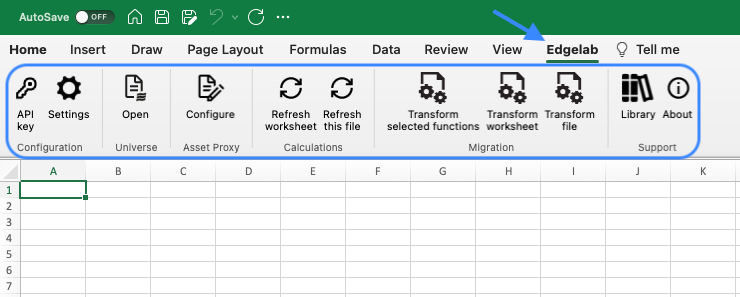
The Edgelab ribbon holds the buttons that allow you to set up your api key, access your Edgelab universe, access templates and stress scenarios identities. From version 24.7 and on, the button Asset Proxy is no longer part of the ribbon.
Configuration group
The Configuration group in the Edgelab tab contains buttons to set up your settings and network proxy choice.
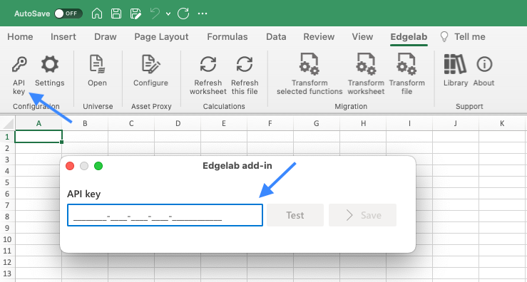
API Key: opens a dialog box to enter the API key and test its authentication. The key can be saved even if its validation fails.
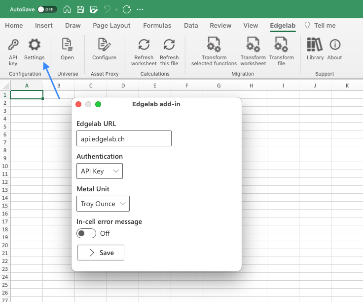
Settings: opens a dialog box to parametrize the network proxy, the authentication method (API KEY or with EL account), the metal unit in which Commodity currency format (e.g. XAU) is expressed. To display the error message directly inside the cell, you can tick the box of In-cell error message. If it is unticked the error message will be displayed when you select a cell with #VALUE!.
Universe group
The Universe group permits you to monitor your Edgelab asset universe
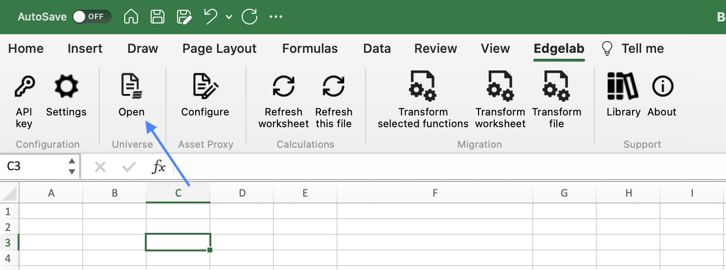
Open: opens the universe portal to access the asset universe. There, you can add and remove assets. UDFs are functional in the frame of the set-up universe. For custom instruments that have been created via our API creations, they need to belong to the universe so that the add-in functions recognize them.
Asset proxy group
The Asset Proxy group embeds the buttons to manage the asset proxy configuration. The mapping of asset proxy within the Edgelab Excel Addin is now deprecated. The mapping should be done via the Universe Portal or via API integration. For further details, do not hesitate to contact our specialists: client.delivery@edgelab.ch.
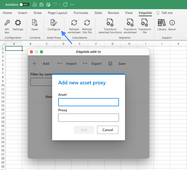
By clicking on Asset Proxy, Configure, the list describe the steps to configure your asset proxy.
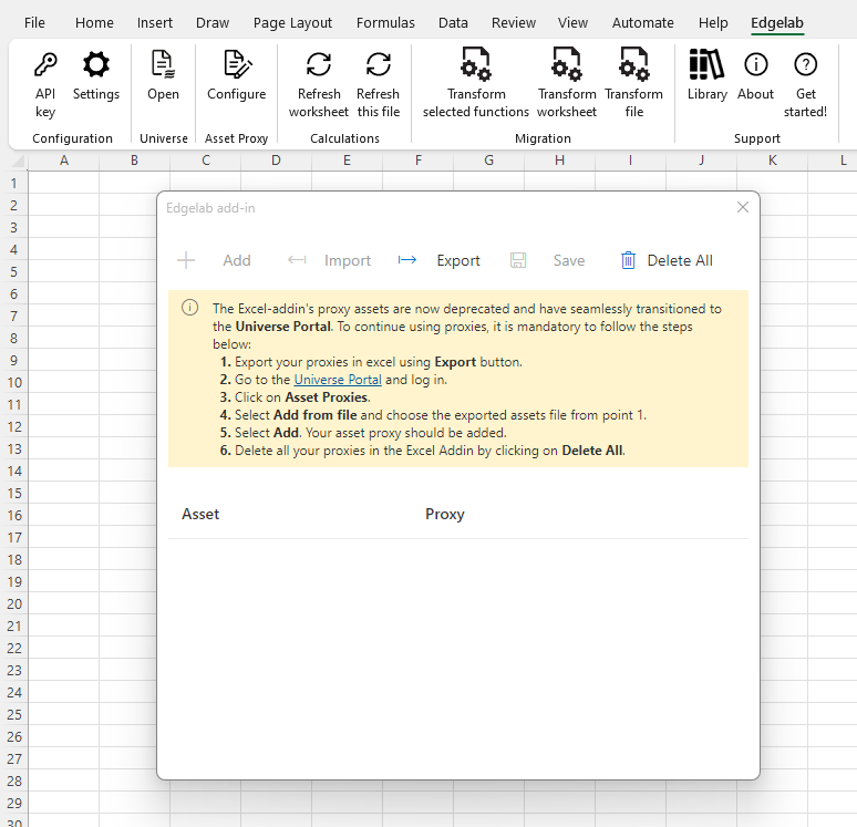
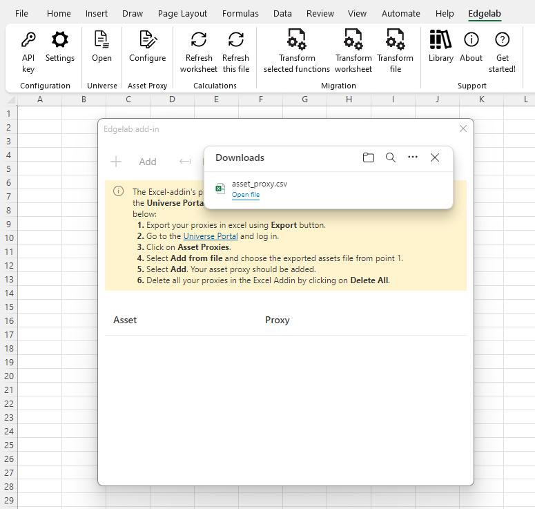
If you had some asset proxy configured in the Add-in, click on Export so you can download the csv. You can then upload it in your Universe Portal.
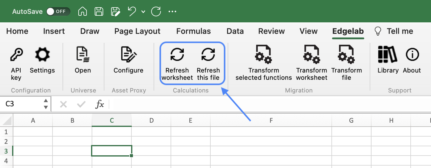
Calculations group
The calculations group in the Edgelab tab contains buttons to refresh one or several sheets in the opened Excel file.
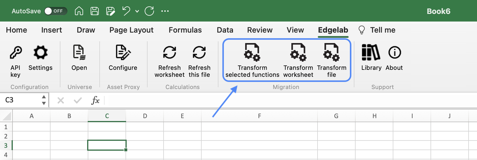
Migration group
The Migration group in the Edgelab tab contains buttons to translate legacy functions into the new format.
Support group
The Support Group in the Edgelab tab contains all the information about the installed version of the Edgelab Add-in.
Library: opens a side panel with templates and stress scenarios documentation.
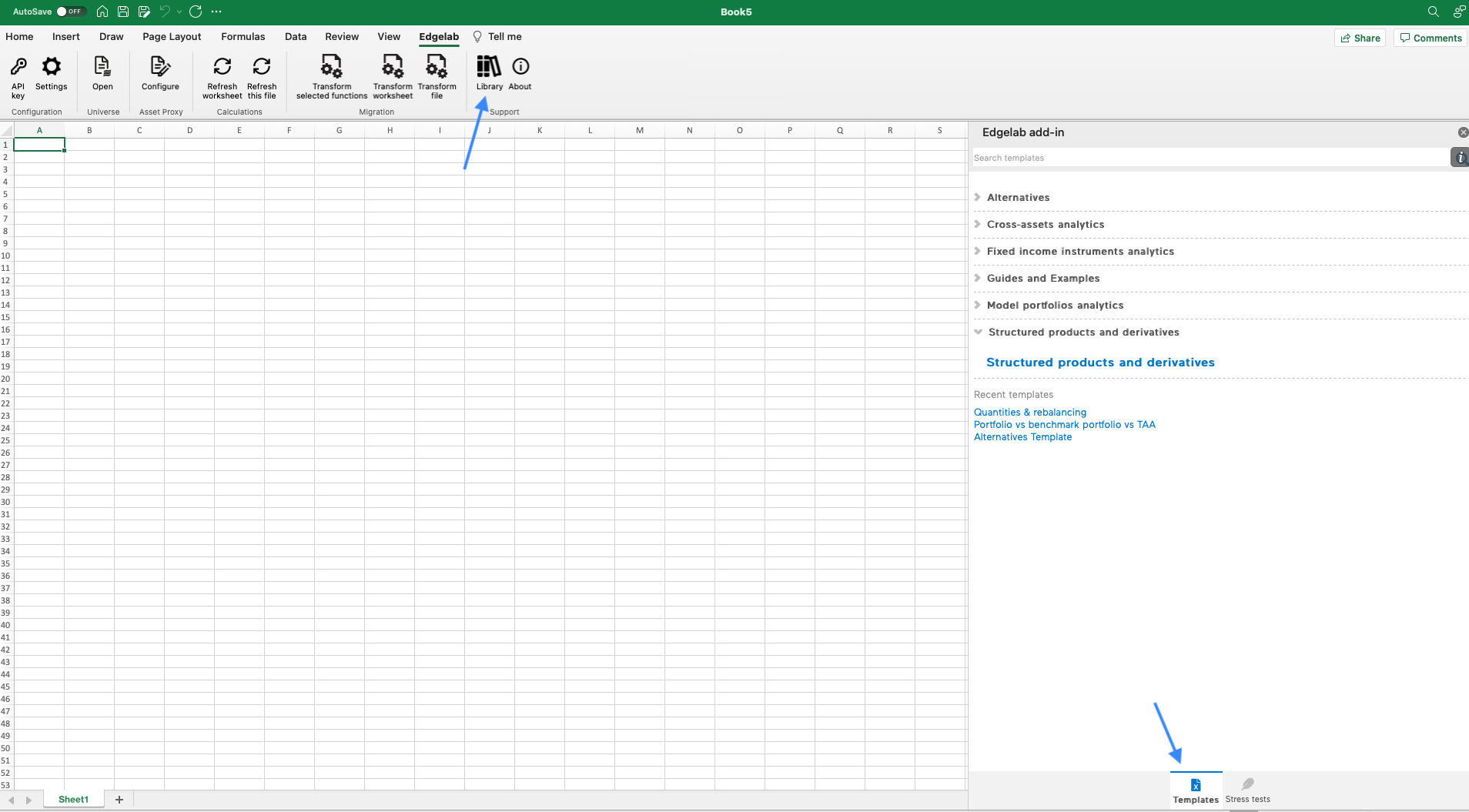
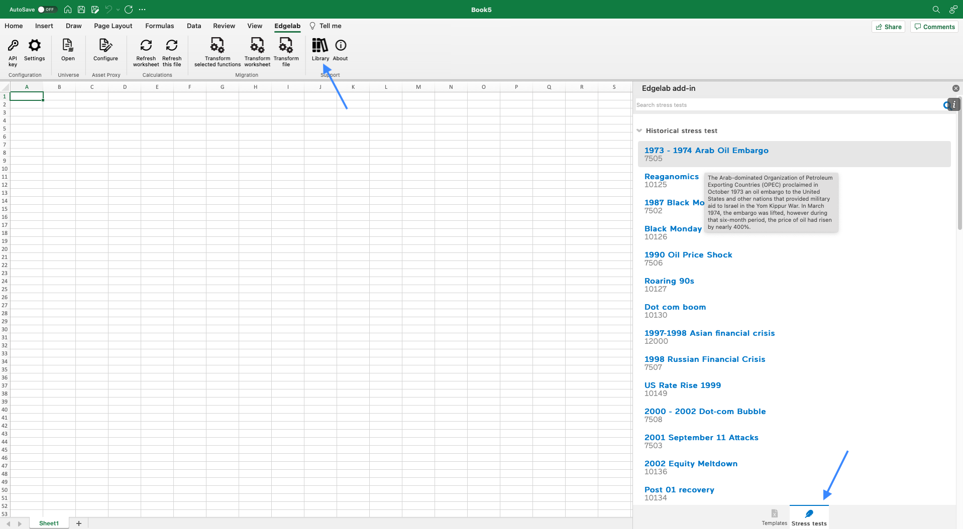
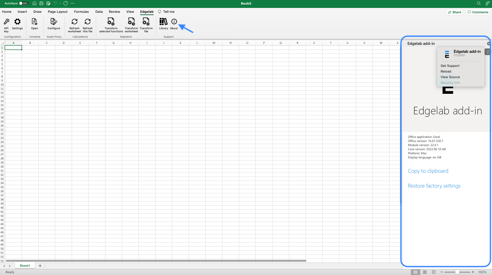
About: opens a window containing a link to the Edgelab website, a link to the Edgelab Add-in documentation, and a link to obtain support. It is also possible to copy the diagnostic information to the clipboard.
